Feynman's sum over paths - a more detailed analysis
Feynman’s methodology
In formulating his theory, Richard Feynman utilised, or one might say more correctly, had a role in formulating himself, the principles of the emerging discipline of Quantum Electrodynamics (QED), the first successful quantum field theory, which also incorporated aspects of special relativity.
What is quantum electrodynamics?
Quantum electrodynamics (QED) mathematically describes all phenomena involving electronically charged particles interacting by means of exchange of photons. In other words, it is a quantum field theory of the classical electromagnetic force affording a complete account of matter and light interaction.
To put this into context, it is necessary to first look at some of the basic principles governing the composition of, and energy levels in, atoms in general and hydrogen in particular[1]:
Energy Levels – the hydrogen atom
In order for a hydrogen atom to exist, it must have both an electron and a proton. The electron has a negative charge and the proton has a positive charge, and these charges work against each other to make the electromagnetic force that holds the entire atom together. They are constantly working against each other because one is positive and one is negative, but their repulsion is what makes the hydrogen atom exist.[2]
Occasionally, the electron will escape from the proton, and if this occurs the hydrogen atom (now a single proton) is said to be positively ionised[3]. Similarly, if a hydrogen atom can sometimes bind another electron to it, such a hydrogen atom is said to be negatively ionised. In astronomy, the former kind of ionisation is much more common.
[1] Unless otherwise indicated, the following material including the graphics accompanying it, are heavily reliant on the very helpful and succinct University of Nebraska-Lincoln Astronomy site: http://astro.unl.edu/naap/hydrogen/levels.html
[2] “How many electrons does a hydrogen atom have?”:
https://www.reference.com/science/many-electrons-hydrogen-atom-d84adcb937b78d13#
[3] Ionisation is the process by which an atom or a molecule acquires a negative or positive charge by gaining or losing electrons to form ions, often in conjunction with other chemical changes. This is succinctly explained by Dawkins and Wong in their wonderful work The Ancestor's Tale, as referenced on the page Particles and forces
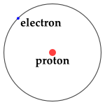
Early and incorrect view of the hydrogen atom. Source: http://astro.unl.edu/naap/hydrogen/levels.html
|
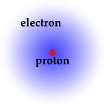
A slightly more accurate view of the H atom. Source: http://astro.unl.edu/naap/hydrogen/levels.html
|
In heavier atoms, the proton is replaced with a mixture of protons and neutrons collectively called the nucleus. The nucleus of the hydrogen atom is just one proton. Helium, on the other hand, has two protons and two neutrons for a total of four nucleons - a general term for particles which are either a proton or neutron.
Because the electron is so much less massive than protons, early physicists visualised the electron as being like a tiny planet which orbited the proton which acted like a tiny sun. Though this view has the advantage of being easy to visualise, it is just an approximate physical representation.
A more physical view of the hydrogen atom is one where the electron is not seen as orbiting the proton like a planet around a sun, but exists as a diffuse cloud surrounding the nucleus. The proton is much stronger than the electron, but it is not necessarily bigger than it. The electron is now shown as a force that encapsulates the entire atom and makes up the majority of the atom, instead of being a simple speck sitting on the edge of the atom.[0]
Only by measuring its location can one know where the electron is (or rather was, as once the electron’s position is measured it moves to a different place). The region where the electron is probably located is called the “electron cloud”. In some cases, the single most probable electron-proton distance happens to correspond to the distance of the more planet-like model.
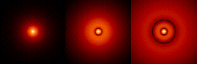
Probability density of the electron for the ground and two excited states of hydrogen. Brighter regions are regions where the electron is more likely to be found. Source: http://astro.unl.edu/naap/hydrogen/levels.html
Orbitals
The density of this electron cloud at any location measures the probability of finding the electron there. In the basic hydrogen atom, shown in the graphic above, the cloud is densest in the centre and thins out with distance from the nucleus, which means the electron is most likely to be found near the nucleus, in a region about 1/20 nm in size[1]. When additional energy is stored in the atom, the electron cloud takes on expanded patterns with low-density “nodal surfaces” corresponding to the dark rings on the right two panels of the figure. These electron cloud patterns are called “orbitals” (a term inherited from the early planet-like visualisation) and each corresponds to a specific amount of energy stored in the atom.
How much energy an electron has determines how far it is way from the proton (or more accurately, how far out the electron cloud extends). Electrons bound to the nucleus cannot have just any value of energy. The electron can only occupy certain orbital “states”, each with a specific amount of stored energy.
There is a lowest energy an electron can have and it corresponds to the state called the “ground state”. When the electron (or atom) has higher energy than this lowest energy, it is said to be in an “excited state”.
Discrete energy levels
Because the states of an electron occur only at discrete energy levels, they are said to be quantised. The electron in a hydrogen atom can only have certain energies. The different energy levels of Hydrogen are denoted by the quantum number n where n varies from 1 for the ground state (the lowest energy level) to ∞, corresponding to unbound electrons.
Excitation
A hydrogen atom with excess energy is said to be “excited“. The two primary ways to excite an atom are through absorbing light and through collisions. When two atoms collide, energy is exchanged. Sometimes, some of that energy is used to excite an electron from a lower energy level to a higher energy level. How many collisions and how energetic the collisions are will depend on how tightly the hydrogen atoms are spaced and their average temperature. Another way to excite an atom is to absorb electromagnetic energy, or in the terminology of quantum mechanics, “absorb a photon”.
The principles governing the process of absorbing or emitting photons[2]
- Because an electron bound to an atom can only have certain energies the electron can only absorb photons of certain energies.
- When an electron drops from a higher level to a lower level it sheds the excess energy, a positive amount, by emitting a photon.
Absorbing a photon
An electron bound to an atom cannot have any value of energy, rather it can only occupy certain states which correspond to certain energy levels.
When an electron absorbs a photon it gains the energy of the photon. Because an electron bound to an atom can only have certain energies the electron can only absorb photons of certain energies. For example an electron in the ground state has an energy of -13.6 eV (electronvolts). The second energy level is -3.4 eV. Thus it would take E2 − E1 = -3.4 eV − -13.6 eV = 10.2 eV to excite the electron from the ground state to the first excited state.
If a photon has more energy than the binding energy of the electron then the photon will free the electron from the atom – ionising it. The ground state is the most bound state and therefore takes the most energy to ionise.
Emitting a photon
Generally speaking, the excited state is not the most stable state of an atom. An electron has a certain probability to spontaneously drop from one excited state to a lower (i.e. more negative) energy level. When an electron drops from a higher level to a lower level it sheds the excess energy, a positive amount, by emitting a photon. [2.1]
Quantum field theory
The quantum field theory approach visualises the force between the electrons as a force arising from the exchange of virtual photons. It is a ‘perturbative’ theory of the electromagnetic quantum vacuum - that is, one that works in approximations, but which can nevertheless be very accurate. QED was the first successful quantum field theory, incorporating ideas such as particle creation and annihilation into a self-consistent framework [3].
QED also incorporates relativity into its predictions, making it a relativistic theory of Quantum Mechanics. Special relativity posits that space and time are aspects of the same thing, known as the space-time continuum, and that time can slow down or speed up, depending on how fast you are moving relative to something else.
Relativistic Quantum Mechanics is therefore applicable to massive particles propagating at all velocities up to those approaching the speed of light, and can also accommodate massless particles, using the general concepts of special relativity and the requirements of quantum mechanics.
Richard Feynman’s work in this area, for which he won a share of the 1965 Nobel Prize, is notable for its accurate predictions. Feynman’s approach consists of two distinct formulations:
- the path integral formulation, and
- the formulation of Feynman diagrams, which came later.
Both formulations contain his ‘sum over histories’ method in which every possible path from one state to the next is considered, the final path being a sum over all the possibilities (also referred to as ‘sum-over-paths’).
The Dirac equation
The Dirac equation formulated in 1928 is a relativistic wave equation, capable of predicting the behaviour of particles at high energies and velocities approaching the speed of light. In quantum field theory (QFT), the equations determine the dynamics of quantum fields. It made "spin" - the particle's angular momentum - a natural property of the electron, postulating "a kind of symmetry, a way of stating mathematically that a system could undergo a certain rotation" [3.1].
In its free form, or including electromagnetic interactions, the equation describes all spin-1/2 massive particles such as electrons and quarks for which parity is a symmetry and is consistent with both the principles of quantum mechanics and general relativity, and was the first theory to account fully for special relativity in the context of quantum mechanics. It accounted for the fine details of the hydrogen spectrum in a completely rigorous way [4]. It also implied the existence of a new form of matter known as antimatter, which was experimentally confirmed several years later (see below), paving the way for the eventual discovery of the positron.
The Lamb Shift
In April 1947, an experiment conducted by Willis E Lamb revealed a minute but significant shift in energy between two energy levels of the hydrogen atom in different states. This phenomenon, which came to be known as the Lamb shift, was not predicted by Dirac’s relativistic wave equation, according to which these states should have the same energy[5]. For his experimental work in this area, Lamb won the Nobel Prize in physics in 1955.
Conflict between experiment and theory
Faced with these experimental results, the problem for theoretical physicists working on this issue was the mathematical tendency of certain quantities of the atom (its mass and charge) to diverge as successive terms of an equation were completed, whereas they should have been vanishing in importance meaning that the closer one stood to an electron, the greater its mass and charge would appear. Under this scenario, a quantity such as the mass of the electron became – if the theory was taken to its ultimate – infinite![6]
By the 1960’s, theorists had managed to work out what was bringing about the existence of different energy levels in the atom. They arose from different combinations of crucial quantum numbers: the angular momentum of the electron orbiting the nucleus and the angular momentum of the electron spinning around itself.
A certain symmetry built into the Dirac equation made it natural for a pair of the resultant energy levels to coincide exactly, but the problem was that that result did not coincide with experiment[7]. Furthermore, the equations had a tendency to produce unwanted and ridiculous infinities.
Renormalisation
It was the Nobel laureate Hans Bethe[8] who offered the first explanation for the Lamb shift in the hydrogen spectrum. He was able to derive the Lamb shift by implementing the idea of mass renormalisation, which allowed him to calculate the observed energy shift as the difference between the shift of a bound electron and the shift of a free electron.
Renormalisation was a process of “adjusting terms of the equation to turn infinite quantities into finite ones. It was”, as Gleick says, “almost like looking at a huge object through an adjustable lens, and turning a knob to bring it down to size, all the while watching the effect of the knob turning on other objects, one of which was the knob itself. It required great care”[9]. Bethe reasoned that something must be missing and hypothesised correctly that it must be the self-interaction of the electron”[10]. His method of getting rid of the infinities was, in essence, simply to pluck a number from the experimental results and to correct, or "renormalise" it, a la a technique first conceived by the Dutch physicist Hendrik Kramers. It was crude but effective. From one perspective, it amounted to subtracting infinities from infinities "with a silent prayer". In Freeman Dyson’s opinion, it was “both a swindle and a piece of genius, a bad approximation that somehow came up with the right answer”[11].
[0] “How many electrons does a hydrogen atom have?”:
https://www.reference.com/science/many-electrons-hydrogen-atom-d84adcb937b78d13#
[1] nm = nanometer, 10−9 m or a billionth of a meter.
[2] This material and that which immediately follows is heavily reliant on another University of Nebraska-Lincoln Astronomy site: http://astro.unl.edu/naap/hydrogen/transitions.html
[2.1] ... and in doing so, the electrons recoil: Gavin Hesketh, The Particle Zoo- The search for the fundamental nature of reality, Quercus, Hachette, London, 2016, 20-21.
[3] See also http://hyperphysics.phy-astr.gsu.edu/hbase/forces/qed.html
[3.1] Gleick, op cit, 229.
[4] See https://en.wikipedia.org/wiki/Dirac_equation and https://en.wikipedia.org/wiki/Relativistic_wave_equations
[5] “Willis E. Lamb, Jr., the Hydrogen Atom, and the Lamb Shift”: http://www.osti.gov/accomplishments/lamb.html; https://en.wikipedia.org/wiki/Lamb_shift
[6] James Gleick Richard Feynman and Modern Physics, Little, Brown and Company, 1992, 231.
[7] Ibid, 239.
[8] He won the 1967 Nobel Prize in Physics for his work on the theory of stellar nucleosynthesis.
[9] Gleick, op cit, 240
[10] Ibid 239.
[11] Ibid, 240.
Feynman's path integral approach - the Lagrangian principle of least action, least time reborn in a quantum context
It was Feynman’s genius that he managed to propound a theory with a sounder base, which envisaged a particle - the electron - following not just one path to get to its final destination but a multitude, indeed an infinity, of possible paths from which it was possible to compute the probability amplitude of a space-time path.
Feynman’s path-integral view of nature, his vision of a sum over histories, was also the Langrangian principle of least action, the principle of least time, reborn in quantum clothing.[1]
Looking at this first of all in classical terms:
|
(w)hy does the moon follow its curved path? Because its path is the sum of all the tiny paths it takes in successive instants of time; and because at each instant its forward motion is deflected, like the apple, towards the earth....The paths of moving objects are always in a special sense the most economical. They are the paths that minimise a quantity called action - a quantity based on the object's velocity, its mass, and the space it traverses. No matter what forces are at work, a planet somehow chooses the cheapest, the simplest, the best of all possible paths....
It is almost impossible for a physicist to take about the principle of least action without inadvertently imputing some kind of volition to the projectile. The ball seems to choose its path. It seems to know all the possibilities in advance.... The behaviour of billiard balls crashing against each other seems to minimise action. So do weights swung on a lever. So in a different way do light rays bent by water of glass.[2] |
Dirac had touched upon these principles in quantum terms some years earlier when he authored an article entitled “The Lagrangian in quantum mechanics” in a somewhat obscure publication entitled Physicalische Zeitschrift der Sowjetunion. Here he worked out the beginnings of a least-action approach as regards the probability of a particle’s path over time in the form of a piece of mathematics for carrying the wave function - “the packet of quantum-mechanical knowledge” - forward in time by an infinitesimal amount: a mere instant. In so doing, he had provided just the germ of a link between the notion of the Lagrangian as envisaged by Feynman and the standard wave function of quantum mechanics as formulated in the Schrodinger equation as a way of expressing a particle’s history in terms of the quantity of action[3], but Feynman needed to carry the wave function farther, through finite time.
Gleick describes the methodology he used[4]:
Gleick describes the methodology he used[4]:
|
Making use of Dirac's infinitesimal slice required a piling up of many steps - infinitely many of them. Each step required an integration, a summing of algebraic quantities. In Feynman's mind a sequence of multiplications and compounded integrals took form. He considered the coordinates that specify a particle's position. They churned through his compound integral. The quantity that emerged was, once again, a form of the action. To produce it, Feynman realised, he had to make a complex integral encompassing every possible coordinate through which a particle could move. The result was a kind of sum of probabilities - yet not quite probabilities, because quantum mechanics required a more abstract quantity called the probability amplitude. Feynman summed the contributions of every conceivable path from the starting position to the final position - though at first he saw more a haystack of coordinate positions than a set of distinct paths. Even so, he realised that he had burrowed back to first principles and found a new formulation of quantum mechanics.
|
:In the end result, Feynman’s path integral formulation generalised the action principle of classical mechanics and replaced the classical notion of a single, unique trajectory for a system with a sum, or functional integral over an infinity of possible trajectories to compute a quantum amplitude to describe the behaviour of the system as a whole, and in so doing, he associated a particle's probability amplitude with its entire motion, that is, with its space-time path. Under this scenario:
The probability for any fundamental event is given by the absolute square of a complex amplitude, and the amplitude for some such event is given by adding together all the histories which include that event[5].
Instead of associating a probability amplitude with the likelihood of a particle’s arriving at a certain place at a certain time – in a wave, largest where the electron is most likely to be found, and progressively smaller at locations where it is less likely to be found[6] - Feynman developed an alternative formulation of quantum mechanics to add to the pair of formulations produced two decades earlier by Schrödinger and Heisenberg, and in so doing he defined the notion of a probability amplitude for a space-time path[7].
Feynman associated the probability amplitude “with the entire motion of a particle” - with a path - the central tenet of his thesis being that in quantum mechanics, the probability of an event which can happen in several different ways is the absolute square of a sum of complex contributions, one from each alternate way. He showed how to calculate the action for each path in complex numbers as a certain integral by adding up all the successive steps taken and squaring the result, hence the term path integral, and established that this approach was mathematically equivalent to the standard Schrödinger wave function, "so different in spirit"[8]. Feynman fully accepted the probabilistic core of quantum mechanics, but offered a powerful new way of thinking about the theory. From the viewpoint of numerical predictions, Feynman’s perspective agrees exactly with all that went before, but its formulation is quite different.[9]
In the classical world, assessing the likely probability of the path of a ball following a succession of baseball hits, for example, is relatively easy, but in Feynman’s quantum world, probabilities are expressed as complex numbers – numbers with both a quantity and a phase, and these so-called amplitudes are squared to produce a probability[10].
In order to find the overall probability amplitude for a given process, then, one adds up, or integrates, the amplitude over the space of all possible histories of the system in between the initial and final states, including histories that are absurd by classical standards. “In calculating the amplitude for a single particle to go from one place to another in a given time, it would be correct to include histories in which the particle describes elaborate curlicues, histories in which the particle shoots off into outer space and flies back again, and so forth. The path integral includes them all. Not only that, it assigns all of them, no matter how bizarre, amplitudes of equal size; only the phase, or argument of the complex number, varies[11].
The path integral: thrown balls and rays of light
|
How does a thrown ball, or - recall - the moon, know how to find the particular arc whose path minimises action? How does a ray of light know to find the particular path that minimises time? Light seems to angle neatly as it passes from air to water. It seems to bounce like a billiard ball off the surface of a mirror. It seems to travel in straight lines. These paths – the paths of least time – are special because they tend to be where the contributions of nearby paths are most closely in phase and most reinforce one another. Far from the path of least time – at the distant edge of a mirror, for example – paths tend to cancel each other out. Yet light does take every possible path, Feynman showed. The seemingly irrelevant paths are always lurking in the background, making their contributions, ready to make their presence felt in such phenomena as mirages and diffraction gratings[12].
|
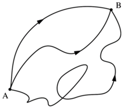 Just three of the paths that contribute to the quantum amplitude for a particle moving from point A at some time t0 to point B at some other time t1. Source: https://en.wikipedia.org/wiki/Path_integral_formulation
In other words, Feynman’s summing of paths, his path integrals, conjures a universe where no potential goes uncounted, where nothing is latent, everything alive and where every probability makes itself felt in the outcome. “The electron does what it likes. It goes in any direction at any speed, forward or backward in time, however it likes, and then you add up the amplitudes and it gives you the wave function”.[13] Feynman had captured the intuitive essence of the two-slit experiment where an electron seems aware of every possibility
Double-slit revisited
Recall for the moment that in the double-slit experiment – the classic example of quantum mechanics in action - waves that pass through both slits interfere with each another. So are they really particles or waves? They can enhance one another or cancel one another, depending on whether they are in or out of phase. Light can combine with light to produce darkness, alternating with bands of brightness, just as water combining in a lake can produce doubly deep troughs and high crests. Each electron “sees” or “knows about” or somehow goes through both slits. Yet if the slits are alternatively closed, so that one electron must go through A and the next through B, the interference pattern vanishes, and if a detector is placed nearby to determine what is in fact going on, the interference pattern is destroyed. Feynman now described these well-established principles quite differently mathematically: as a combination of all the paths and histories a particle can take in arriving at its ultimate destination.
Recall for the moment that in the double-slit experiment – the classic example of quantum mechanics in action - waves that pass through both slits interfere with each another. So are they really particles or waves? They can enhance one another or cancel one another, depending on whether they are in or out of phase. Light can combine with light to produce darkness, alternating with bands of brightness, just as water combining in a lake can produce doubly deep troughs and high crests. Each electron “sees” or “knows about” or somehow goes through both slits. Yet if the slits are alternatively closed, so that one electron must go through A and the next through B, the interference pattern vanishes, and if a detector is placed nearby to determine what is in fact going on, the interference pattern is destroyed. Feynman now described these well-established principles quite differently mathematically: as a combination of all the paths and histories a particle can take in arriving at its ultimate destination.
Waviness, Feynman explained, was built into the phases carried by amplitudes, like little clocks. He was really eliminating the wave viewpoint altogether: the field was a quantised manifestation of the particle, but the actors were more than ever particles[14].
Compare this to the quantum phenomenon of superposition of states:
Compare this to the quantum phenomenon of superposition of states:
|
At the quantum scale, particles can also be thought of as waves. Particles can exist in different states, for example they can be in different positions, have different energies or be moving at different speeds. But because quantum mechanics is weird, instead of thinking about a particle being in one state or changing between a variety of states, particles are thought of as existing across all the possible states at the same time. It’s a bit like lots of waves overlapping each other… If you’re thinking in terms of particles, it means a particle can be in two places at once. This doesn’t make intuitive sense but it’s one of the weird realities of quantum physics.
However, once a measurement of a particle is made, and for example its energy or position is known, the superposition is lost and now we have a particle in one known state[15]. |
Random and stochastic, but probable processes
The path integral also relates quantum and stochastic processes – processes having a random probability distribution or pattern that may be analysed statistically but not predicted precisely. Because stochastic processes are random and therefore unpredictable, one must therefore rely on probabilities, probabilities which are nevertheless extremely accurate in predicting outcomes in this area.
[1] For the enunciation of Lagrangian principle which follows, see Gleick, op cit, 57-61.
[2] Ibid, esp 69-61.
[3] Gleick, op cit, 128-9.
[4] Op cit, 131-2.
[5] http://academickids.com/encyclopedia/index.php/Path_integral_formulation
[6] Brian Greene, The Elegant Universe, Vintage, 2000, 106.
[7] Gleick op cit, 246 ff
[8] Ibid, 247-8.
[9] Greene, op cit, 108.
[10] Gleick, op cit, 247.
[11] http://academickids.com/encyclopedia/index.php/Path_integral_formulation
[12] Gleick, op cit, 250. A diffraction grating consists of a plate of glass or metal ruled with very close parallel lines, producing a spectrum by diffraction and interference of light
[13] Feynman to Freeman Dyson, Ibid, 250.
[14] Gleick, op cit, 250..
[15] http://www.physics.org/article-questions.asp?id=124
The role of antimatter
At a time when Feynman struck an impasse in his thinking, he fell back once more on Dirac’s equation which had thrown up the existence of a new form of matter known as antimatter. Dirac’s picture of the vacuum was a lively sea populated by occasional holes or bubbles. If an electron fell into a hole and filled it, both the hole and the electron would disappear. In due course, a gamma ray (nothing more than a high frequency particle of light), could spontaneously produce a pair of particles: one electron and one positron. Dirac suggested that negative energy levels did exist but were normally already occupied by electrons, and because of Pauli’s exclusion principle, no ordinary positive energy electron can make a transition to any of these levels[1]. Dirac’s relativistic equation thus presupposed negative energy giving rise to antimatter.
According to Dirac, by shining light on the contents of an empty box, which is in fact full of energy, we should be able to excite one of the negative energy electrons to a positive energy level, and we would then have a positive energy electron together with a ‘hole’ in the Dirac sea of negative energy electrons which would in turn have positive energy and positive charge. The result would be the creation of an electron-positron pair by a photon. The positron is the antiparticle of the electron – a particle with the same mass but opposite charge. The positron was found by Carl Anderson in 1932, four years after Dirac wrote down his equation. It looked like an electron, but travelled up through a magnetic field when it should have travelled down[2].
Feynman’s refinement: particles travelling backwards in time and particle pair creation
To avoid the unwanted infinities sometimes resulting from Dirac’s equation, Feynman proposed a forward and backward flowing version of time, and a space-time picture in which the positron was a time reversed electron, and with the aid of a student came up with some vivid imagery in support:
|
A bombardier watching a single road (by analogy, the path of the electron) through the bomb-sight of a low flying plane suddenly sees three roads, the confusion only resolving itself when two of them move together and disappear and he realises he has only passed over a long reverse switchback (zig-zag) of a single road. The reversed section represents the positron in analogy, which is first created along with an electron and then moves about and annihilates another electron.
|
Hey and Walters come up with an even more graphic illustration, describing imaginary electron paths on a pin ball table and comparing them with those on a contiguous graphic depicting the electrons in space and time:
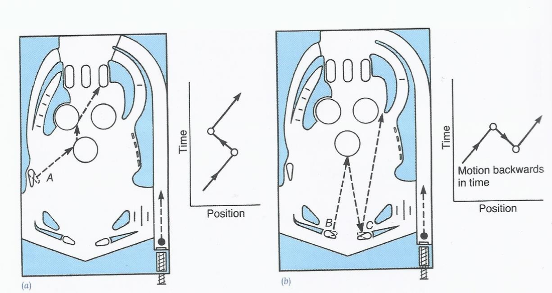
Source: Hey and Walters, The New Quantum Universe, Cambridge University Press, 2003, page 234.
 The basic Feynman diagram “The fundamental interaction”. Source for graphic and explanation: See Gleick, op cit, 274.
The motion of the electrons in a spatial direction corresponds to movement across the table. Motion up the table corresponds to the time evolution of the electron’s trajectory. The attempt on the left is normal both in space and time, but on the right the electron appears to have been scattered (propelled) downwards, that is, backwards in time.
Working off Dirac’s equation, according to Feynman, in relativistic quantum mechanics, this possibility was allowed if the electron going back in time had negative energy and this corresponds to electron-positron pair creation. The positron then travels forward in time to the second scattering centre where it is annihilated by the original incoming electron. Feynman realised that diagrams with ‘backwards in time’ electron paths could be understood as the physical process of pair creation followed by pair annihilation. Negative energy electrons travelling backwards in time correspond to positive energy positrons travelling forwards in time. According to Hey and Walters, this ‘backwards in time’ concept is but a device to avoid having to use the complicated machinery of quantum field theory, for “as far as we know, nothing actually travels backwards in time”![3]
Feynman diagrams[4]
The calculation of probability amplitudes in theoretical particle physics requires the use of rather large and complicated integrals over a large number of variables, which if unleashed tend to result in a mass of algebraic computations. These integrals do, however, have a regular structure, and may be represented graphically as Feynman diagrams – pictorial representations of the mathematical expressions describing the behaviour of subatomic particles in spacetime.
A Feynman diagram consists of points, called vertices, and lines attached to the vertices, and the particles are allowed to go both forward and backward in time. Fermions (matter particles and their antiparticles, such as electrons and positrons) are represented by straight lines. Bosons ("messenger" particles), such as photons, are depicted by means of wavy lines. In each diagram, time is represented along one axis and space along the other: the positron is depicted as an electron moving backward in time and antiparticles generally are represented as moving backward along the time axis. Each point of intersection indicates an interaction between two particles, but is also a type of shorthand notation for a series of (often highly complicated) equations.[4.1]
The meeting points for the lines can also be interpreted forward or backwards in time, so that if a particle disappears into a meeting point, that means that the particle was either created or destroyed, depending on the direction in time that the particle came in from. All the lines and vertices have an amplitude. When you multiply (1) the probability amplitude for the lines, (2) the amplitude for the particles to go from wherever they start to wherever they meet, and to the next meeting point, and so on, and (3) also multiply by the amplitude for each meeting point, you get a number that tells you the total amplitude for the particles to do what the diagram says they do. If you add up all these probability amplitudes over all the possible meeting points, and over all the starting and ending points with an appropriate weight, you get the total probability amplitude for a collision in a particle accelerator, which tells you the total probability of these particles to bounce off one another in any particular direction.
To recapitulate, a Feynman diagram is a space-time diagram, in which the progress of time is shown upward on the page. If one covers the above diagram with a sheet of paper and then draws the paper slowly upward:
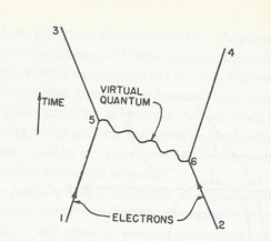
The role of virtual photons and amplitude calculation in the diagram
The diagram depicts the ordinary force of repulsion between two electrons as a force carried by a quantum of light. Because it is a virtual particle [4.2], coming into existence for a mere ghostly instant, it can temporarily violate the laws that govern the system as a whole, in other words the exclusion principle or the conservation of energy. The diagram is therefore an aid to visualisation, but it serves physicists mainly as a book-keeping device. Whatever carries force can move only as fast as light. In the case of electromagnetism, it is light itself – in the form of these fugitive “virtual” particles that flash into existence just long enough to help quantum theorists balance their books, repaying the energy which has been borrowed for the short period of time necessary for these particles to briefly flirt into existence and then disappear again. Each diagram is associated with a complex number, an amplitude that is squared to produce a probability for the process shown[5].
Feynman noted that it is arbitrary to think of the photon as being emitted in one place and absorbed in another. One can say just as correctly that it is emitted at (5), travels backwards in time, and is then (earlier) absorbed at (6). Each diagram represents not a particular path, with specified times and places, but a sum of all such paths. Each diagram could replace an effective lifetime of Schwingerian algebra[6].
Here is another Feynman diagram, depicting a contribution of a particular class of particle paths, which join and split as described by the diagram:
- A pair of electrons – their paths shown as solid lines – move towards each other.
- When (6) is reached, a virtual photon (described below) is emitted by the right hand electron (wiggly line), and the electron is deflected outward.
- At (5), the photon is reabsorbed by the other electron, and it too is deflected outward.
The role of virtual photons and amplitude calculation in the diagram
The diagram depicts the ordinary force of repulsion between two electrons as a force carried by a quantum of light. Because it is a virtual particle [4.2], coming into existence for a mere ghostly instant, it can temporarily violate the laws that govern the system as a whole, in other words the exclusion principle or the conservation of energy. The diagram is therefore an aid to visualisation, but it serves physicists mainly as a book-keeping device. Whatever carries force can move only as fast as light. In the case of electromagnetism, it is light itself – in the form of these fugitive “virtual” particles that flash into existence just long enough to help quantum theorists balance their books, repaying the energy which has been borrowed for the short period of time necessary for these particles to briefly flirt into existence and then disappear again. Each diagram is associated with a complex number, an amplitude that is squared to produce a probability for the process shown[5].
Feynman noted that it is arbitrary to think of the photon as being emitted in one place and absorbed in another. One can say just as correctly that it is emitted at (5), travels backwards in time, and is then (earlier) absorbed at (6). Each diagram represents not a particular path, with specified times and places, but a sum of all such paths. Each diagram could replace an effective lifetime of Schwingerian algebra[6].
Here is another Feynman diagram, depicting a contribution of a particular class of particle paths, which join and split as described by the diagram:
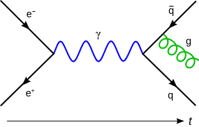
In this Feynman diagram, an electron and a positron annihilate, producing a photon represented by the blue sine wave) that becomes a quark-antiquark pair, after which the antiquark radiates a gluon (represented by the green helix) . Source: See https://en.wikipedia.org/wiki/Feynman_diagram
Again: the points in Feynman diagrams where the lines meet represent two or more particles that happen to be at the same point in space at the same time. The lines in a Feynman diagram represent the probability amplitude for a particle to go from one place to another. These diagrams are very simple in QED, where there are only two kinds of particles: electrons (little particles inside atoms) and photons (particles of light). In QED, the only thing that can happen is that an electron (or its antiparticle) can emit (or absorb) a photon, so there is only one building block for any collision. The probability amplitude for the emission is very simple - it has no real part, and the imaginary part is the charge of the electron[7].
Feynman's mental picture for these diagrams started with the hard sphere particle approximation, and the interactions could be thought of as collisions at first. It was not until decades later that physicists thought of analysing the nodes of the Feynman diagrams more closely. The world-lines of the diagrams have since become tubes to better model the more complicated objects such as strings and M-branes[8].
Recapitulation with the aid of explanatory allegories
To recapitulate, the essence of Feynman's sum-over-paths (sum-over-histories) approach is built upon the presupposition that a particle can travel between two points A and B by a - possibly infinite - number of different paths, and each one of these paths will have a certain probability associated with it.
A visual depiction of what occurs is has been advanced in terms of having friends who live about 10 minutes' walk away: “When they come to our house, they are a few different routes they could take - one is definitely the most obvious and direct, and there are a few other routes they could take if they wanted without going too far out of their way”.
Alternatively they could take any number of more indirect routes, go by the local gelato shop or even via Melbourne if they choose to do so. The probability of them doing that is very small indeed, but it's still not zero because if they want to, they can.
“Nevertheless, we don't know for sure which route they are going to take from their house to ours - all we can do is assess the probabilities that they'll take each route, and make our guess based on that. So each route between their house and ours has a non-zero and non-one probability assigned to it, and the sum of all the probabilities is one. When they reach our house, they tell us which route they took. In doing that, the probability that they took that route becomes one, and the probability that they took all the others becomes zero”.
The author[9] describes this as an analogy to the situation where a particle must take every possible path between two points, but when you check which path it took, it appears that it only took one of them. “Each path has its own probability from the vanishingly small - eg. a photon travelling from the Sun to the Earth via the Andromeda Galaxy - to the very likely, which would be the photon following the straightest possible geodesic between the two points. In other words, one assumes that particles are taking every possible route until you check which route they are actually taking”.
Similar scenarios have been advanced as regards a traveller entering a railway station via one of many available entrances, with equally as many exits. What are the probabilities of him exiting via any one of these? These examples may suffice as an aid to understanding except that visitors travelling between houses and train travellers entering and exiting a railway station manifest themselves as individuals in the classical world, whereas, as another observer points out [10], the essence of the sum over paths approach in the quantum world is that each available path will have a different probability amplitude but with a wavelike nature.
|
“As these waves spread through space they interfere with each other, their respective wave patterns either reinforcing or cancelling each other out at various points. And if you sum over all the amplitudes of all the different paths, i.e. if you sum-over-histories, then the different amplitudes will reinforce or cancel each other in such a way that the only path that survives this interference process is the one that the particle actually follows”. [11] So in quantum mechanical terms, these probabilities are encoded in the wave function that describes the particle, which assigns to each possible path a different probability amplitude, the square of which gives the corresponding probability.
|
Does Feynman's 'all possible paths', replete with particles visiting outer space before returning to travel through the other slit, violate special relativity and its dictum of light-speed as a maximum?
No. As Gleick points out in his commentary on Feynman's "fundamental interaction" diagram, force cannot be transmitted instantaneously: "As Feynman's diagrams automatically made explicit, whatever carries force can move only as fast as the speed of light. In the case of electromagnetism, it is light - in the form of fugitive "virtual" particles that flash into existence just long enough to help quantum theorists balance their books". [12]
Furthermore:
[1] Tony Hey and Patrick Walters, The New Quantum Universe, Cambridge University Press 2003, 228-9; Gleick, op cit, 253.
[2] The antiproton – the antiparticle of the proton – was not discovered until 1955 at Berkeley, California in 1955, and had to await the arrival of the Bevatron accelerator to do so.
[3] Op cit, 235. However, more recently, scientists from the University of Queensland, Australia, have used single particles of light (photons) to simulate quantum particles travelling through time, demonstrating in the process that one photon can pass through a wormhole and then interact with its older self: http://www.ibtimes.co.uk/physicists-prove-time-travel-possible-by-sending-particles-light-into-past-1453839; http://www.collective-evolution.com/2015/12/07/physicists-send-particles-of-light-into-the-past-proving-time-travel-is-possible/ Their findings were published in Nature Communications.
[4] Except where otherwise indicated, this material consists of an edited summary of Gleick, op cit, 270-277.
[4.1] Adam Hart-Davis, Science - The definitive visual guide, London, 2009, 327.
[4.2] The nature and role of virtual particles in the context of Heisenberg's uncertainty principle is considered on the page Something out of nothing - again
[5] Gleick, op cit, 273-274.
[6] Julian Schwinger was a contemporary physicist and one of Feynman’s rivals in this field. His calculations and methodology were far more complex than those of Feynman. “Feynman’s approach was original and intuitive, while Schwinger’s was formal and laborious”: Gleick, 268. Nevertheless, Feynman and Schinger shared the 1965 Nobel prize for their respective contributions to the development of quantum electrodynamics in this field along with the Japanese physicist Sin'ichirō Tomonaga.
[7] https://simple.wikipedia.org/wiki/Feynman_diagram
[8] http://www.spaceandmotion.com/Physics-Richard-Feynman-QED.htm
[9] Matthew Lancey, qualifications disclosed in https://www.quora.com/What-is-Richard-Feynmans-sum-over-paths-approach-to-quantum-mechanics
[10] Steve Denton, ibid.
[11] Ibid.
[12] Gleick, op cit, 273.
[13] This is a summary of principles drawn from:
No. As Gleick points out in his commentary on Feynman's "fundamental interaction" diagram, force cannot be transmitted instantaneously: "As Feynman's diagrams automatically made explicit, whatever carries force can move only as fast as the speed of light. In the case of electromagnetism, it is light - in the form of fugitive "virtual" particles that flash into existence just long enough to help quantum theorists balance their books". [12]
Furthermore:
- The scenario about particles following all possible paths is basically a method of calculation and is not intended to be taken literally. "It certainly is not true that the particle really can travel faster than the speed of light and be anywhere in the universe".
- The path integral formalism works out the correct result even though it includes non-physical paths (including extreme paths such as those which purport to travel down to the local cafe and elsewhere in the universe) because all the non-physical paths will cancel each other out completely. In summary, it is a calculational technique and it does not mean that particles really do take all possible paths to get from point A to point B.
- These methods imply that every photon "knows" about every possible path and it calculates the probability of each path... "You just have to accept it. The equations are super-wacky but they give results accurate to 12 decimal places, so just accept it. Somehow, each little bit of nothing senses around awhile lot of space and does the equivalent of trillions of calculations. Just live with it. That's all you can do. Don't try saying "it's illogical". It works. We are going onto 65 years since Feynman's methods came out, and though illogical, they work". [13]
[1] Tony Hey and Patrick Walters, The New Quantum Universe, Cambridge University Press 2003, 228-9; Gleick, op cit, 253.
[2] The antiproton – the antiparticle of the proton – was not discovered until 1955 at Berkeley, California in 1955, and had to await the arrival of the Bevatron accelerator to do so.
[3] Op cit, 235. However, more recently, scientists from the University of Queensland, Australia, have used single particles of light (photons) to simulate quantum particles travelling through time, demonstrating in the process that one photon can pass through a wormhole and then interact with its older self: http://www.ibtimes.co.uk/physicists-prove-time-travel-possible-by-sending-particles-light-into-past-1453839; http://www.collective-evolution.com/2015/12/07/physicists-send-particles-of-light-into-the-past-proving-time-travel-is-possible/ Their findings were published in Nature Communications.
[4] Except where otherwise indicated, this material consists of an edited summary of Gleick, op cit, 270-277.
[4.1] Adam Hart-Davis, Science - The definitive visual guide, London, 2009, 327.
[4.2] The nature and role of virtual particles in the context of Heisenberg's uncertainty principle is considered on the page Something out of nothing - again
[5] Gleick, op cit, 273-274.
[6] Julian Schwinger was a contemporary physicist and one of Feynman’s rivals in this field. His calculations and methodology were far more complex than those of Feynman. “Feynman’s approach was original and intuitive, while Schwinger’s was formal and laborious”: Gleick, 268. Nevertheless, Feynman and Schinger shared the 1965 Nobel prize for their respective contributions to the development of quantum electrodynamics in this field along with the Japanese physicist Sin'ichirō Tomonaga.
[7] https://simple.wikipedia.org/wiki/Feynman_diagram
[8] http://www.spaceandmotion.com/Physics-Richard-Feynman-QED.htm
[9] Matthew Lancey, qualifications disclosed in https://www.quora.com/What-is-Richard-Feynmans-sum-over-paths-approach-to-quantum-mechanics
[10] Steve Denton, ibid.
[11] Ibid.
[12] Gleick, op cit, 273.
[13] This is a summary of principles drawn from:
- http://physics.stackexchange.com/questions/20823/does-path-integral-and-loop-integral-in-a-feynman-diagram-violate-special-relativity
- https://www.quora.com/Quantum-theory-says-a-particle-can-be-anywhere-in-the-universe-in-the-next-instant-Photons-are-the-fastest-particle-but-are-limited-to-the-speed-of-light-How-can-both-be-true - an excellent answer by Frank Heile, PhD in Physics from Stanford University
- http://motls.blogspot.com.au/2010/10/dont-mess-with-path-integral.html, also described as The Reference Frame
